Image processing

The branch related to computer graphics is image processing. Repeatedly the created images are subjected to additional processing in order to get effects hard to obtain directly by the use of computer graphics methods. In this lecture we will learn selected methods in the scope of image processing.

The starting point in image processing is source image in the bitmap form. The goal is to get another version of this image somehow better from the user point of view. There exist many methods of image processing. In general several groups may be distinguished. These are: geometric transformations, point transformations, filtering, spectral transformations, morphological transformations. Here we limit the considerations to the first three groups.

The geometrical transformations usually concerns the whole images. Typical transformations are translation, revolutions, mirroring. Here we include also cropping that enables choosing specific fragment from the image. The examples of such operations are shown in Fig. X.1. Frequently we want to apply operation only to the fragment of image. To indicate such fragments we use different types of masks.

Fig. X.1. Examples of operations on the whole bitmap. a) Original image, b) revolution through 90°, c) horizontal mirroring, d) skewing along x axis, e) revolution through an α angle, f) cropping

Some of operation done on the whole image (or on chosen fragment) are algorithmically simple the others are more complex. Please think for a moment about realisation of counter clockwise rotation through 90° as shown in Fig. X.1b. We can notice that we may perform this operation as follows. We change an order of pixels in each row, and then swap the rows and columns (see Fig. X.2).

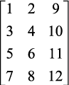
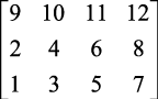
Fig. X.2. Counter clockwise rotation of pixel matrix through 90°

The revolution of bitmap through an angle different than 90° or 180° angle is more complex operation. The general procedure is shown in Fig. X.3. At first we rotate the pixel matrix through given angle. Then we set the target mesh of pixels and for each target pixel we find these pixels from rotated original matrix that are covered be considered target pixel. Then we define the level of coverage of rotated pixels. This level defines the weight of influence of covered pixel onto the final colour of target pixel.

Fig. X.3. Bitmap rotation through an angle α

Let us notice that in such type of transformations as bitmap rotation we must perform operations related to particular pixels of initial image, whereas in vector graphics we transform objects that means their vertices or control points.

Point transformations concerns specific pixels of image independently on the state of neighbouring pixels. The examples of such operations are creation of the negative of an image, change of image using transfer characteristic, tresholding (binarisation), pseudocolouring. The results of operations are shown in Fig. X.4.

Fig. X.4. Results of chosen single point operations: (a) original, (b) negative, (c) tresholding, (d) pseudocolouring, (e) change intensity levels, (f) transfer characteristic

In single point transformation we perform given operation with respect to each pixel independently. The details of operation usually are described by look up table giving the resultant value associated with particular entry. The other way is to define a transfer function that assign new values to the pixels of specific intensities.

Look up table is used for example for changing the colours of an image. Each location in this table contains new colour which should substitute specific colour from original image. For example to the pixel of grey level 11 we should assign green colour, and for pixel with grey level 127 the red colour should be assigned. Such type of image transformation is named pseudocolouring. It is shown in Fig. X.4d. In particular the look up table may describe only the colour swapping in the scope of original set of colours of initial image.

The required type of transformation may be defined by the function that transform specific original values into new values. For the purpose of obtaining negative of image with grey scale we may use the function such as L’ = 255 – L, where pixels intensities: original L and new L’ are binary coded in the range from 0 to 255. Different types of functions may be used: power, exponential, logarithmic, monotonic and non monotonic or individually chosen for particular processing task. For example the image from Fig. X4f was obtained From an image in Fig. X.4a using the function from Fig. X.5a. In particular case the function may be such as shown in Fig. X.5b. Then all the intensity levels lower than the threshold are change into black colour and all levels with value greater than threshold are changed into white colour. In such case we get black and white bi-level image and the operation is called image thresholding (see Fig. X.4c).

Fig. X.5. Example of transfer functions defining changes of pixel intensities. On horizontal axis there are intensities before transformation on vertical axis the intensities after transformation a) Function for image from Fig. X.4f, b) threshold function.

The next group contains transformations that use pixel neighbourhood. Such operations are done using appropriate filters or masks. The operation is done on each pixel of original image. The result is stored in new target image. The principle of operation is shown in Fig. X.6.

Fig. X.6. Illustration of the processing method using filter 3 × 3. The intensity of pixel in target image is defined on the base of pixels forming neighbourhood of given pixel

The mask (filter) is a table of elements, usually square with dimension 3 × 3, 5 × 5 etc. Particular elements of table are weighting coefficient that are multiplied by the values of neighbourhood pixels. The value of new pixel is calculated from the equation

$$p_(x,y)={∑↙{i,j=-m}↖m w_{ij}\;p_{x+i,y+j}}/{∑↙{i,j=-m}↖m w_{ij}}$$

where coefficients $w_{ij}$ are elements of square filter of size $2m + 1$, $p_{x,y}$ is processed pixel , while $p_{x+i,y+i}$ are the pixels from neighbourhood in a square of size $2m + 1$. If the sum of weighting coefficients is equal to 0 or to 1 the final pixel value is calculated from equation

$$p_(x,y)=∑↙{i,j=-m}↖m w_{ij}\;p_{x+i,y+j}$$

Let us notice that the pixels belonging to the first and the last row of image must be treated in different way. In the simplest case we just omit these pixels. In most complex case we use another filers with the size 2 × 3 for this rows.

The type of the operation depends on the applied mask. There are many different filters known. In particular we distinguish low pass filter that enables removing of small distortion in the image (by averaging, which results in some kind of blurring the image), high pass filters that exaggerate the edges present in the image (sharpen the image) and filters that detect the edges. In Fig. X.7 some examples of filters are shown, while in Fig. X.8 example of results are shown.

Fig. X.8. The results of filter application: a) original image, b) low pass filter, c) high pass filter, d) edge detection

In image processing the notion of image histogram is used. Histogram is a diagram, in which for each colour (grey level) existing in an image the number of pixels having this colour is given. These number are represent as vertical line segments of appropriate height. The image and its three R, G and B histograms are shown in Fig. X.9.

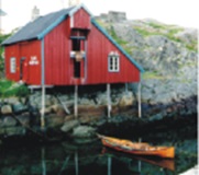
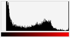
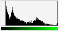
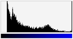
Fig. X.9. a) Image b) its histograms for R, G and B colours

At the end let us pay attention to the fact that in image processing there exist some model images, that are use for testing the efficiency of different algorithms. One of such images is an image called "Lena" originally in colour, the grey level version also exists (Fig. X.10). The results of a few further image processing operations will be shown using this image.

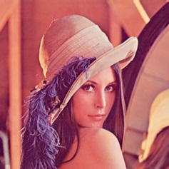
Fig. X.10. Model image of Lena

In Fig. X.11 a few versions of Lena image are shown. In fig. a) the image with gamma correction with gamma value equal to 2.2 is shown. Such correction is used to compensate distortions introduced by non-linear characteristics of CRT displays. In fig. b) the posterisation effect is shown, which is the result of too small number of available grey levels. In fig. c) noisy version of image is shown. In fig. d) the effect of edge detection in the image is shown.

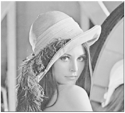
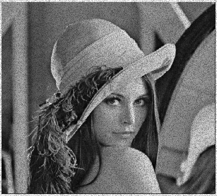
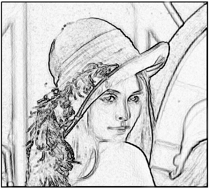
Fig. X.11. Examples of image modification. a). Gamma correction, b) posterisation, c) noisy image, d) edge detection

In Fig. X.12 examples of image distortions are shown.

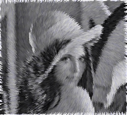
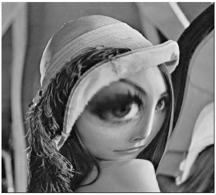
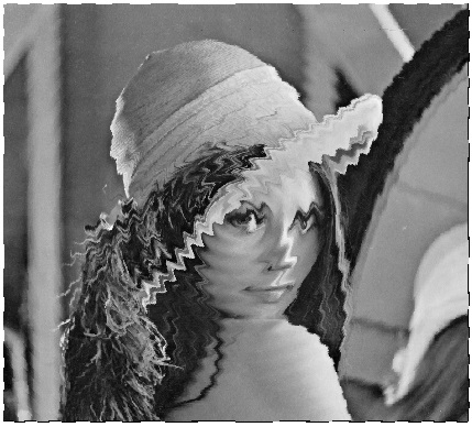
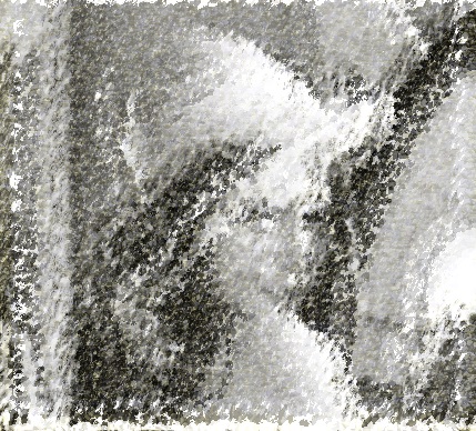
Fig. X.12. Examples of image distortions

In Fig. X.13 two examples of modifications by insertion of another images are shown.

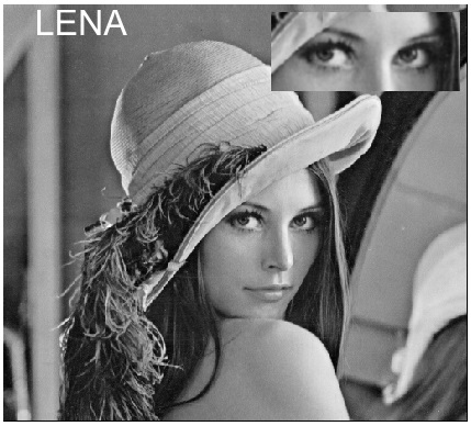
Fig. X.13. Examples of modification of image content

Professional image processing program offer great number of another operations on digital images.