Animation

Creation of animating films has a long history. In natural way the appearance of computers caused fast development of animation. In this lecture selected problems characterising methods of using computers in animation are presented.

Up to now we deal with creation of a single - static image. But the surrounding reality is not static and the computer graphics methods should enable solving the problem of visualisation of changes occurring in time. This is the field of computer animation. In animation a set of frames (still images) reflecting the view of the scene in next discrete moments. In turn due to some inertia of our visual system when the series of frames are displayed with sufficient frequency we get the impression of fluency of changes occurring in time.

It is worth noting that the animation is not limited only to the movement - each change between next frames is some form of animation. So, for example, change of the shape of the object or change of the look of the object are some forms of animation. Let us notice that during displaying a sequence of images, the next images may be treated as samples of continuous sequence of real events, taken at specific time intervals. The sequence of frames that form animation is created off-line and then it may displayed with required frequency.

The concept of computer animation is similar to classic animation when the main animator drew by hand key frames for animated sequence and assistants drew on this basis a set of intermediate frames. In computer animation the main animator uses appropriate computer graphics application programs to draw key frames. The computer create intermediate frames.

In creation of animation, for the parameter whose values changes in time, key frames must be distinguished. For these frames the animator must set the value of parameter. The values for intermediate frames are calculated by computer using chosen interpolation method, linear or non-linear, between values from key frames.

Frequently the values of many parameters are changing in time, not necessary at the same moment. Then it is convenient to store information about the moments of change in summary diagram, for example such as shown in Fig. IX.1. Six parameters are taken into account. For each of them key frames are marked with respective colour point.

Fig. IX.1. The demonstration of notation of information about moments, where the values of particular parameters change. Points with specific colour mark key frames for given parameter

In Fig. IX.2 the example of finding third intermediate frame for the triangle changing its placement between first and fifth key frames with the use of linear interpolation. Let us notice that interpolation is done on the vertices of the triangles. It means that the placement of vertices in key frames was defined earlier.

Fig. IX.2. Example of finding the intermediate frame

At first we connect corresponding points (vertices of both triangles) with line segments. Than using the linear interpolation method, the placement of points for intermediate frames is defined. For simplicity Fig. IX.2 shows only one intermediate frame K3 lying in the midpoint between frames K1 and K5.

In general during moving object we must take into account interpolation of object placement, interpolation of object rotation, controlling the speed of movement, interpolation of other object parameters.

At first it is always important to define a path along which the change of parameter takes place. This path must be defined on the base of knowledge of parameter P values in next key frames (Fig. IX.3). After defining the path we are able to calculate the values of parameter P in intermediate frames.

Fig. IX.3. Example of path of object movement defined by the values of parameter P in key frames

In general the path may be curvilinear. In the example form Fig. IX.3 the path was defined be a curve interpolating points from key frames. Hermite's curves may be used for example. These are third order curves containing Hermite's arcs. Each Hermite's arc connects two neighbouring points with known placement and derivative vectors. It is possible also to control the speed and the acceleration of movement of object along chosen path.

During movement of object along the path it may rotate simultaneously. The problem of angle interpolation between initial and ending angles defined in key frames arises. It occurs that classic method of calculation of rotations with the use of appropriate matrices sometimes fail. This effect may appear when during calculations two from three axes of coordinate system will be in one line (align), what leads to so called gimball lock. To avoid this phenomenon for rotation interpolation we use the most frequently the quaternion calculus. It is based on Euler thesis on rotations according to which it is possible to transit from any given angle orientation to any another by means of single revolution about certain axis. In particular the axis may go through the origin of coordinate system. Using quaternions we have the warranty to avoid gimball lock effect.

One of more difficult objects that can be met at creation of animation is human figure. In the case of modelling of human body as a rule at first the skeleton is modelled. Then the flesh and a skin are stretched on it. The skeleton is constructed from stiff solids connected by rotational joints or ball joints. Control of movements of human body (skeleton) is a hard task due to number of joints and many limitations. For this reason in practice we use the motion capture method. Let us assume that in animation a character should make a sequence of movements. It is possible to hire an actor and place a set of appropriate markers or sensors in different places on his body. Then, when the actor performs the assumed sequence of movements, the subsequent placements of markers or sensor are registered as time flows. On the base of registered information it is possibly to reproduced the movement of animated person accurately. In similar manner we can solve the problem of the animation of facial expression.

Object moving in scene may collide with other objects. In correct animation the collision should be detected and the adequate action should be undertaken. The definition of the time of collision is not obvious. It results from the fact that the frames are separated by some time interval. So in the first frame there is no collision yet and in the next it is after collision and the object already started to penetrate into another object. Allowing the situation of penetration of one object into another is not the best solution. Thus it is better to assume that collision occurs earlier than it really does. Knowing the distance between the objects and their velocities we may estimate when the collision will take place and accept the frame preceding this fact as a moment of collision.

During testing the collision the method of testing whether the collision really took place is important. Let us explain it on the example of two moving cubes. At first glance it seems that it is sufficient to test whether any of vertices of one cube is located inside the other cube as in Fig. IX.4a. But we must take into account the situation in Fig. IX.4b. None of vertices of the first cube is inside the second cube, but the collision took place already.

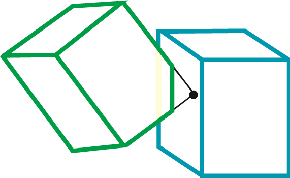
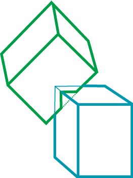
Fig IX.4. Illustration of collision testing

After finding collision we must define the behaviour of collided objects. The reaction method depends on many factors. In most cases it necessary to comply to the laws of physics. For example the ball thrown up after some time falls onto earth surface. We have to define initial direction of flight and speed and also calculate the height of flight using well known equation describing the movement of the body in gravity field. If it bounces from the ground it should not fly higher than previously.

One of the animation techniques is deforming the objects (morphing) that means change of shape of the objects (sometimes the notion of warping is used). In the simplest case we may use geometric transformations with respect to vertices of figures or solids, or with respect to curve control points (for example Bezier curves) or curvilinear surfaces.

Simple method of shape modification relies on shifting one vertex of the object and propagation this shift to neighbouring vertices with gradual decrement of the size of shift. The example is shown in Fig. IX.5.

Fig. IX.5. Example of shape modification

In described example we deal all the time with the same object - only its shape was changing. In another type of animation we may meet the transformation of one object into another object. We speak about metamorphosis or just morphing. In Fig. IX.6 simple example of morphing is shown, which is gradual transition from blue figure to yellow figure along given curve.

Fig. IX.6. Example of morphing between objects shown in fig. a) along the given curve in fig. b)