Rasterisation algorithms

Line segments

Let us introduce the problem. The goal is to draw a line segment with known coordinates of both endpoints. In Fig. IV.a the look of line segment that we are used to and which can be obtained on paper using a pencil and a ruler is shown. In Fig. IV.b the look of the same line segment drawn on raster basis is shown. In this example we deliberately chose very small raster resolution in order to clarify the problem. Then we chose arbitrarily the pixels included in line segment.

Fig. IV.1. a) Ideal look of line segment b) line segment drawn in raster

Let us think about the algorithm enable choosing pixels for line segment with given endpoints coordinates. Let us assume that x, y coordinate system is associated with our raster. It is known that if we know the endpoint coordinates of line segment, it is possible to derive the equation describing the line containing given line segment. We remember the form of this equation

$$y=mx+b$$

where m is a factor defining slope $m=\tan α$ and α is an angle between X axis and the line - slope angle. Knowing line equation we may proceed as follows. For the next raster column at $x_i$ coordinate it is possible to calculate from line equation the value of $y_i$ coordinate of the point lying on the line. Then it is possible to find the closest raster node in column $x_i$. It is explained in Fig. IV.2 The procedure should be repeated for each column in terms of changes of x coordinate for whole line segment.

Fig. IV.2. Finding next pixels with the use of line equation

The method is simple. But for finding placement of next pixel it is necessary to perform operation of multiplication, adding and rounding. The number of executed operation may be reduced if we notice that at constant slope and constant distance between columns equals to1, the value of $y_{i+1}$ in next column $x_{i+1}$ can be calculated adding to the value $y_i$ constant increment $Δy=m$. Using the dependency

$$y_{i+1}=y_i+m$$

to calculate next pixel placement it is necessary to execute one floating point addition and one rounding. Thus we spare one multiplication. If we take into account that during generation of single image sometimes it is necessary to draw several dozens of line segments each containing several dozens of points it occurs that sparing in terms of the number of executed calculations become significant. And we remember that time for calculation the next image is always very short. This version of algorithm is called DDA algorithm.

Let us notice that the described way of acting is right at assumption that the slope is not greater than 45°. At the angle greater than 45° and less than 90° it is necessary to introduce a modification and now we will define pixels in subsequent rows instead in columns as previously. Without this change the number of pixels lying on line segment may become to small, what is illustrated in Fig. IV.3a.

Fig. IV.3. Line segment with slope greater than 45°. a) set of pixels chosen along columns - erroneous variant b) set of pixel chosen along rows - correct variant

It occurs that it is possible to further reduce calculation time of line segment drawing, adding the requirement to use only fixed point operations only and not floating point operations as it was in case of DDA algorithm. Suitable algorithm was elaborated by Bresenham.

Before we present full Bresenham algorithm let us see the reasoning that resulted in final form of the algorithm. We assume the slope of line less than 45° (i.e. $0<m<1$). Let us assume that the pixel in column $x_i$ has been found already and we should find the pixel in next column $x_{i+1}$. It may be noticed that the choice is limited to two pixels: the one lying in the same row and another lying in the row above. (see Fig. IV.4.). So it remains only to find simple criteria for choosing the pixel at the smallest computational effort. Bresenham proposed to design such criteria using the difference of distances D1 and D2 between considered pixels and the point lying on real line segment (see Fig. IV.4). It may be noticed that the pixel may be chosen by testing the sign of (D1 – D2) difference. If negative we choose upper pixel, if negative lower pixel.

Fig. IV.4. Illustration of Bresenham reasoning. Candidate pixels to be chosen in next column are marked in green

Finally the Bresenham algorithm looks as follows:

1. Knowing line segment endpoints coordinates we should choose the endpoint with lower x coordinate. (Because algorithms not always gives the same result when starting from different endpoint the rule was accepted to start always from the endpoint with lower value of x coordinate). Chosen point $(x_1,\,y_1)$ is the first point of drawn line segment.
2. Calculate auxiliary values:

   

   and initial value of decision parameter p as:

   

3. For next columns with $x_k$, coordinate, starting from $k=0$ the sign of decision parameter $p_k$ should be tested

   In the case of $p_k<0$ next pixel has coordinates $(x_{k+1}, y_k)$ and new value of decision parameter is defined from dependency $p_{k+1}=p_k+a$.

   In the opposite case next pixel has coordinates $(x_{k+1}, y_{k+1})$ and new value of decision parameter is defined from dependency $p_{k+1}=p_k+b.$

4. Step 3 is repeated until we get to the end of line segment.

Let us notice that in each step in order to find next pixel we should execute single fixed point addition.

Example

Using Bresenham method find next pixel for line segment with endpoints coordinates (2,2), (8,5).

1. We choose first point of line segment. It is point (2,2).
2. We calculate auxiliary values $$\table Δx=8-2=6, Δy=5-2=3, a=2∗3=6, b=6-12=-6$$ $$p_0=2Δy-Δx=6-6=0$$

3. Finding next pixels

   Because $p_0=0$, the next pixel has coordinates (3,3) and $p_1=p_0+b=0-6=-6$

   Because $p_1<0$, the next pixel has coordinates (4,3) and $p_2=p_1+a=-6+6=0$

   Because $p_2=0$, the next pixel has coordinates (5,4) and $p_3=p_2+b=0-6=-6$

   and so on. The whole line segment is shown in Fig. IV.5.

Fig. IV.5. Example of results of Bresenham algorithm

Aliasing

The appearance of line segment drawn on raster certainly is not the best. Especially for not very high raster resolution it can be clearly seen that the shape of line segments deviates from ideal - stair case effect can be seen. The situation becomes even worse when the line segment is rotated with respect to given pivot point. During slope changing the pattern of pixel placements also changes. In Fig. IV.6 sample line segments with different slope are shown.

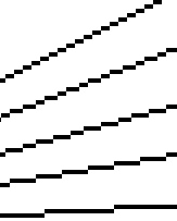
Fig. IV.6. Sample line segments with different slope

Described effect is called aliasing. It results from finite raster resolution. Effect cannot be removed by any method. But it is possible to reduce it. Methods serving such goal are named antialiasing.

The overbearing solution is increase of resolution. The tendency to increase display resolution has been keeping for long years and now the aliasing effects are less noticeable. But although we frequently do not notice aliasing effect it still exists and we may be convinced enlarging the image from display screen, for example during projection onto big wall screen. The effect is illustrated in Fig. IV.7. Left side shows the view from display screen. Right side shows enlarged line segment with visible pixel structure. Some antialiasing method was applied to this line segment. Watching the enlarged version of line segment we may notice that particular pixels have different grey levels.

Fig. IV.7. a) Line segment b) enlarged fragment of line segment

The principle of applied method relies on choosing two pixels closest to ideal line in each column. Dependent on the distance between pixel and point on a line grey levels are assigned to these pixels - the closer is the pixel to point on line the darker it becomes. The sum of grey levels is constant. In the case of pixel lying close enough to point on line, single pixel is displayed in the column. Described method is illustrated in Fig. IV.8

Fig. IV.8. Illustration of method of aliasing effect reduction, where two pixels are displayed in each column

Antialiasing method may be used directly during the rasterisation of objects contours. In practice frequently another solution so called full screen antialiasing is used. After generation of full pixel image antialiasing method is applied to the whole image. Typically it is FSAA method. The image is generated in greater resolution than target resolution. During reduction to target resolution the averaging of colours of neighbouring pixels takes place.

Circle

Now let us consider how can we draw a circle with center at the origin of coordinate system and radius r. Obviously we may use circle equation $x^2+y^2=r^2$ and for next values $x_i$ calculate in each column the values of y and after rounding find appropriate pixels. Such method is computationally expensive (there is squaring and square rooting). Moreover placement of pixels approximating the circle is not uniform (please wonder why). Thus in practice another methods are used. Below mid point method is presented.

At first we may notice that during finding pixels that approximate the circle we may use circle symmetry features. It allows to limit pixel calculation to one octant (one eighth of circle). The remaining pixels are found according to the principle shown in Fig. IV.9

Fig. IV.9. After finding the point marked in red, the points marked in green are found using circle symmetry features

Let us explain the idea of center point method. At first let us remember that each point lying on the circle fulfils the equation $x^2+y^2-r^2=0$. For point outside the circle the inequality $x^2+y^2-r^2>0$, holds, and for points inside the circle the inequality $x^2+y^2-r^2<0$ becomes true. In turn if we consider only the first octant of the circle then after finding the pixel in column $x_i$, in next column $x_{i+1}$ the choice is limited to two pixels: one lies in the same row the other lies in the row below (see Fig. IV.10). Center point is the point lying in the middle of line segment connecting two candidate pixels. The choice between candidate pixels is done by analysing the placement of center point with respect to the circle. If the center point is inside the upper pixel is chosen, when it is outside we choose lower pixel. It occurs that in circle drawing, similarly to drawing a line segment by Bresenham method, it is possibly to find a criteria for pixel choice that requires only execution of a few simple operations.

Fig. IV.10. Illustration center point method

Finally the algorithm of drawing a circle with center at the origin of coordinate system and radius r looks as follows:

1. Starting point has coordinates (0, r). The initial value of auxiliary decision parameter is equal to $p_0=5/4-r$

2. For next columns with coordinates $x_k$, starting from $k=0$, the sign of auxiliary decision parameter $p_k$. should be tested

   In the case of $p_k<0$, next pixel has coordinates $(x_{k+1}, y_k)$ and a new value of decision parameter is calculated from equation $$p_{k+1}=p_k+2x_{k+1}+1.$$

   In opposite case the next point has coordinates $(x_{k+1}, y_{k-1})$ and a new value of decision parameter is calculated from equation $$p_{k+1}=p_k+2x_{k+1}+1–2y_{k+1}.$$

3. Remaining seven pixels are found using circle symmetry features

4. The steps 2 and 3 are repeated until fulfilling the condition $x=y$.

I propose to make it for Your own. Find pixels for the circle with center at origin of coordinate system and radius $r=20$.

Other curves and figures

Having available line segment drawing algorithm we may solve the problem of polyline and polygons drawing. The examples of such objects are shown in Fig. IV.11. Let us notice that the lines and contours may have assigned different attributes such as style(continuous, interrupted, dotted), thickness or colour.

Fig. IV.11. Sample objects constructed from line segment with different attributes

Such computationally simple algorithms as for line segments and a circle exist for a small number of other objects (for example for an ellipse). In the case of other curves described by equation, usually it is necessary to use this equation for finding y coordinate value for next x coordinate values and then rounding to the closest pixel coordinates. In some cases we may use symmetry features (for example for sinusoidal curve).

Frequently we do not know the equation of needed curve. Then interactive drawing of such curve remains. No always it is convenient method. In such cases we may use special type of polynomial curves for example Bezier curves (see next lecture).

Rasterisation inside closed contours

Closed contours frequently required finding pixels lying inside the contour. Two methods may be distinguished for such rasterisation: scan line method and starting point - seed method.

Scan line method

In scan line methods we assume that the equations describing contour are known. There are two stages in such methods. In first stage, for each raster row the crosspoints of row and contour are found. Then the pairs of crosspoints, between which we should make filling, are found. In the next stage drawing horizontal line segment found in the first stage takes place. In Fig. IV.12 sample raster lines crossing polygon and marked crosspoints with the edges of polygon are shown. In second stage the line segments limited by the pairs of points P₁ (1,2), P₂ (3,4), P₃ (5,6) will be drawn.

Fig. IV.12. Finding the line segments contained in polygon interior which will be filled in second stage of scan-line algorithm

The concept of algorithm is simple and it does not cause significant implementation problems in the case of convex polygons. In particular implementation for defined class of objects, for example for nonconvex polygons, we must pay attention to the vertices. Usually it is necessary to distinguish two classes of vertices. In first class both edges lie at the same side of raster line (in other words these are vertices which are local extremum). In second class the edges lie at the opposite sides of raster line (see Fig. IV.13).

Fig. IV.13. Two types of vertices

Starting point method

In this group of methods we assume that the closed contour is drawn on the screen and the point belonging to contour interior is known. Filling starts from known point belonging to the interior of figure.

Sample order of conduct may be as follows. Beginning from starting point we move left along the raster line until we meet the border of the area. Then in the same row we move right from starting point until we meet the border of area. Then we go up and repeat the procedure starting from the point lying above the starting point. We repeat these steps as long as it is possible. Then we go to the row lying below the row containing starting point and proceed in similar way as previously. We may also create and actualise the list of active pixels - these who lie on the edge of already filled area. Then if we need, we may continue the procedure from the first pixel found in active pixels list etc.

In Fig. IV.14 intermediate stage of filling is illustrated. Starting point is marked in blue colour. Black marks already found pixels belonging to contour interior. Pixels from the list of active pixel are marked in green.

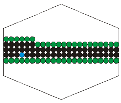
Fig. V.14. Illustration of starting point method. Filling starts from the point marked in blue colour

Let us notice that the algorithm is capable to fill convex polygon as well as nonconvex or even non consistent.

Triangle rasterisation

Special case of filling is rasterisation of the triangle with known vertices. It obviously may be done by one of the methods described above.

In practice we frequently use so called barycentric coordinates (see below). If we find barycentric coordinates of specific pixel, then testing of the signs of these coordinates we may tell whether the pixel is inside (all coordinates are positive) or outside the triangle (at least one coordinate is negative).

Barycentric coordinates

Barycentric coordinates define the placement of point inside the triangle of known coordinates of vertices. (Fig. IV.15).

Fig. IV.15. Sample triangle with internal point distinguished

Let us assume that coordinates of triangle vertices are respectively A, B, C. Placement of point U inside the triangle is described by coordinates α, β, γ

U = αA + βB + γC

such that

α + β + γ = 1   i   α, β, γ≥0

Barycentric coordinates may also be used for linear interpolation of the values of function inside the triangle.

Let us assume that the values of certain function at triangle vertices A,B,C, respectively f(A),f(B),f(C) are known and we know the barycentric coordinates of point U inside the triangle. Then the value of function in point U is equal to

$$f(U)=αf(A)+βf(B)+γf(C)$$

Finding pixel colours

In rasterisation process there is a problem with finding the colours of pixels. In the case of lines or contour edges the colour is set in advance and all pixels have this colour assigned.

In the case of pixels belonging to the contour interior we may applied different variants of filling. The interior may be filled uniformly with the same colour (constant filling), with varying colour (tonal filling or shading) or with the texture. Example of filling effects are shown in Fig. IV.16.

Fig. IV.16. Examples of figure interior filling: a) constant colour, b) tonal, c) texture

In constant filling all internal pixels get the accepted in advance colour. In texture filling internal pixels have assigned colours „taken” respectively from used texture pattern (problems concerning textures are presented in Lecture VIII). As it concerns tonal filling we will limit ourselves to present Gouraud method for the triangle case.

Let us assume that we know colours (or intensity values) of each triangle vertices and we want to find the colour of each pixel inside the triangle.

Let us consider left edge of the triangle (see Fig. IV.17). Let us mark the intensities of vertex colour by $I_1$ and $I_2$. This edge is crossed by raster lines. Knowing the values $I_1$ and $I_2$ we are able to find the interpolated intensity for each crosspoint of edge with raster line using linear interpolation method. Similarly for right edge of triangle with vertex intensities $I_1$ and $I_3$ we may find the colours of intermediate points lying on the edge. In turn let us consider a part of raster line belonging to the triangle. Because we know already the intensity values at the endpoints of this line segment ($I_a$ and $I_b$ on Fig. IV.17), we are able, similarly to triangle edges, to find intermediate values for specific pixels belonging to part of raster line inside the triangle (for example the value $I_c$ in a figure. Proceeding that way for next raster rows we may find the intensity of each pixel inside the triangle. In effect we get tonal shading of the surface of the triangle. Examples of such shading are shown in Fig. IV.17 for grey level version and for colour version.

Fig. IV.17. Gouraud method. a) Illustration of principle of the method b,c) example of obtained effects

Certain limitation of Gouraud method is that the set of colours obtainable for triangle interior is limited by the set of the colours of vertices.

Calculations in Gouraud method may be also done with the use of barycentric coordinates. If we know the colours of triangle vertices c₀, c₁, c₂ then the colour of pixel c_p with barycentric coordinates α, β, γ may be found from equation

$$c_p=αc_0+βc_1+γc_2$$