Image storing

Lossless compression

Just the simplest method of lossless compression is a method of coding the series of characters known as RLE method. The essence of this method relies on finding a sequence of identical elements and storing their value and number of occurrence repetition. Let us assume that the pixels in monochrome image (with grey levels) are represented on bytes and a series of pixel in the image is such as in Fig. XI.1a. This series may be written according to given rule in the way shown in Fig. XI.1b. In each pair of the numbers the first means repetition number and the second the value of pixel. It is obvious that having compressed sequence and remembering the rule of compression we are able to perform decompression and restore accurately original series of pixels.

Fig. XI.1. The example of RLE compression method. a) Information before compression, b) compressed information

Effectiveness of RLE compression is great when the long series of the same values appears. However if there are single values then instead of profit, the losses may occur. (In some implementation the solutions for such special cases are included). Usually, in particular implementations we compress separate rows of the image. It is not a general rule. There exist solutions where the columns of image are coded, or a sequences chosen by ZigZag method (see Fig. XI.4).

Let us pay attention to colour images coding. If the pixel is represented using three primary colours R, G and B, then the image may be written as a sequence of RGB triplets representing next pixels. But it also may be written as three separate sequences each containing only one primary, respectively only R component, only G component, and only B component of next pixels (see Fig. XI.2). It may be noticed that in the second case the effectiveness may be greater, due to the greater chance to meet longer series of identical values in the series of the same component (forming so called R, G and planes).

Fig. XI.2. The influence of data ordering on effectiveness of compression. a) pixel order, b) order according to component colours

In general the RLE compression method allows the compression levels in the range 2 : 1, 3 : 1. Obviously the compression level depends on given image - fore some images it may greater and for the others may be less. It is a characteristic feature of all compression methods.

Among the other methods of lossless compression methods the Huffman method should be mentioned, where the codes of different length are used. For the pixels most frequently appearing in the image shorter codes are assigned.

The method works as follows. At first we test how many pixels in the image has specific colour (for example by preparing image histogram). Then the percentage of participation is ordered from the greatest to the smallest value and an auxiliary tree is created. Among the ordered percentage participation of colours we find two values which has minimal value of a sum. They are joined and founded sum is assigned to the created tree node - the component values forming the sum are removed. The procedure is repeated for the remaining set of values. Tree creation ends when we get to the root. After creation of tree, in each tree node we assign values 0 or 1 to the edges. Then starting from the root we find the shortest paths leading to the leafs. For each path the values assigned to the edges are registered. The obtained series of binary values are the codes which in compression process will be assigned to the colours associated with specific tree leaf.

During the compression process we scan next pixels of the image and assign new codes to them. The codes are added to compressed sequence. Let us notice that in most cases the original pixel code (for example 8 bit) is substituted by shorter code. It is important that for the pixels with most frequent colours the shortest codes are assigned. The resultant compressed code should be necessarily equipped with coding table.

Decompression process is simple. We look at compressed series from the beginning and test whether the bit sequence corresponds to any code from code table. If so in restored image we place original pixel colour before compression. The procedure is repeated until full original image is restored. In the whole process compression - decompression no information is removed. Obtained compression levels are in the range a few to one.

Example

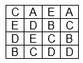
Compress with Huffman method the image shown below. Pixels are coded on 8 bits.

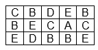
Let us start from finding the histogram.

Then we create Huffman tree and find new codes for particular pixels.

Then we prepare compressed image sequence and add the coding table

011110110111110010000110001101110
A-000, B-11,C-01,D-001,E-10

Notice. In this simple example compression level is small - not taking into account the code table is equal approximately to 2.

Spośród innych metod kompresji bezstratnej należy wymienić metodę słownikową LZW. Istotną cechą tej metody jest to, że w czasie kompresji obrazu jest równocześnie zapisywana informacja o słowniku i nie potrzeba go niezależnie dołączać do postaci skompresowanej. Słownik ten jest odtwarzany stopniowo czasie dekompresji. Ponieważ metoda LZW była przez wiele lat objęta ochroną patentową, to często wykorzystywano w praktyce wcześniejszą wersję tej metody LZ77, która nie była objęta ochroną patentową.

Lossy compression

One of the most frequently used lossy compression methods is JPEG. It is very complex method, so we will present only the general concept of this method. At first the image is divided into sub-images (blocks) of the size of 8x8 pixels. Each block undergoes the compression independently. The stages of compression process are shown in Fig. XI.3.

Fig. XI.3. Block diagram of JPEG compression method

In the first step the conversion from RGB model to model YCbCr (digital version of the model YUV) takes place. The next steps of algorithms are made independently for luminance component Y and for chrominance components Cb and Cr. Calculations for luminance Y are done with greater accuracy than for Cb, Cr components – we use the fact that human eye is more sensitive to luminance changes than to the change of colour.

For the block of values of luminance Y with the size 8×8 we perform cosine transformation and as a result we get new set of 64 numbers - coefficient of cosine development. The following equation is used:

$$S_{vu}=1/4C_uC_v∑↙{x=0}↖7∑↙{y=0}↖7 s_{yx}\cos{(2x+1)uπ}/16\cos{(2y+1)vπ}/16$$

where $s_{yx}$ are the original data from the table with coordinates yx and $S_{vu}$ are coefficients obtained as the results of cosine transformation written in the table with coordinates vu. Coefficients $C_u$ and $C_v$ are equal to $1/√2$ when $u,v=0$ and equal to 1 in the opposite case.

In next step so called quantisation is done. The purpose is to exchange as great as possible number of coefficients of transformation for zero. In general the point is that among the coefficients of transformate there are such that convey great number of information about the image and such that convey very little information. The lasts may be eliminated without significant loses in general image quality. Their influence is so small, that the observer may even do not notice the changes in image due to removal of this coefficients.

The quantization is done in the following way. We use auxiliary table 8x8 containing properly chosen values. Then in turn we divide the coefficients from the table obtained during transformation by corresponding coefficients from auxiliary table. The first element from the table of coefficients of transformation is divided by the first element from auxiliary table, then the same is done to second elements and so on. The results are down rounded. The elements in auxiliary table are chosen in such way, that in resultant table possible great number of zeroes grouped in the lower right corner of resultant table appear. Due to quantisation we obtain compression of the information. The operation is not reversible.

The table obtained as a result of quantisation is subjected to coding by RLE method and then Huffman coding. The series of values from resultant table is scanned in ZigZag order and coded by RLE method what is shown in Fig. XI.4. Such order is accepted for the purpose of obtaining long series of zeroes grouped in lower right corner of the table. Let us notice that the series does not include the element from the upper left corner marked as DC It is coded parallel with respective elements for another 8x8 blocks that the image under compression consists of.

Fig. XI.4. Scanning of table elements in ZigZag order

During decompression we act in reverse order. At first we perform Huffman decoding, then the RLE decoding. The restored table is subjected to reverse operation with respect to quantisation (with the use of auxiliary table) it is obvious that we can not restore the coefficient that were zeroed. The restored table of coefficient of cosine transformation is subjected to reverse cosine transformation. Finally the conversion from YCbCr model to RGB model is performed.

The JPEG compression method achieves compression levels 20:1 – 30:1, with practically invisible distortions of the image restored after decompression. At greater compression levels the changes become visible. (The compression level change is obtain by changing the coefficients of an auxiliary table used in quantisation process). It is shown in Fig. XI.5 where the image of Lena was compressed 20 :1 and 50:1. The images after compression are shown at right side, upper and lower place respectively. At the lower left side the difference image between original and the image after decompression 20:1 is shown. Here we can see the information that was removed in compression - decompression process.

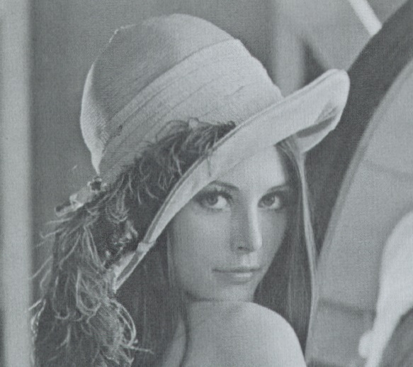
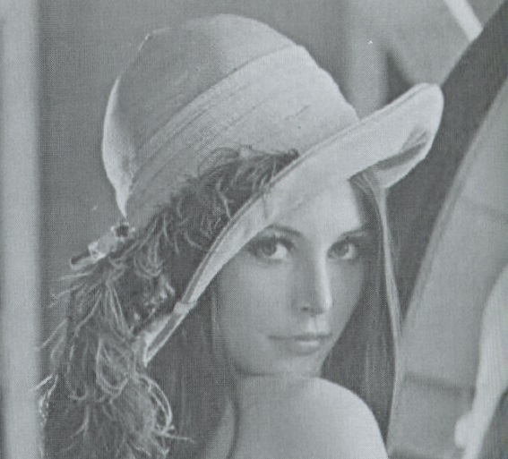
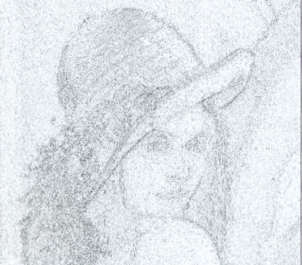
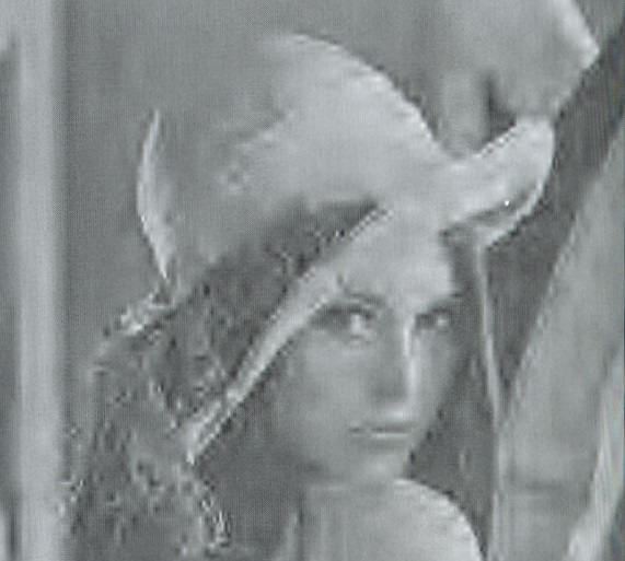
Fig. XI.5. a) Image of Lena, b) image compressed 20:1 after decompression, d) image compressed 50:1 after decompression, c) difference image between image a) and b)

Above the basic version of JPEG standard, most frequently used in practice is presented. In fact full standard includes 29 different compressions including the lossless compression. In 2000 year the next version of compression JPEG2000 was developed, where it was assumed that the compression is done directly on the whole image and wavelet transformation is used. But this standard was not accepted in practice.

At the end we add that the discussed above compression methods are applied for compression of single still images. During compression a sequence of images (such as animation) the different methods are used for example such as in MPEG standards.