Rendering

Viewing pyramid

Defined scene may be observed from different locations. Observer may be placed at any point of the scene, usually it is assumed that the observer is outside the objects. Moreover observer can look at any direction. Depending on observer placement and direction of view the respective view of a scene should appear on the screen. It is explained demonstratively in Fig. VII.1 (for simplification top view is shown). It is assumed that the observer's viewing angle α is constant.

Fig. VII.1. Observer's placement and direction of view determine elements of the scene visible to observer. Two example of observer placement A and B are marked along with viewing directions

In the A position of the observer object 5 will not appear on the screen, objects 1, 2 and 4 will be only partially visible and object 3 probably will not be visible, because it is obscured by the objects lying closer to the observer. In the B position of the observer object 5 will not be visible, all remaining object will be only partially visible.

Some conclusions may be drawn from the analysis of the figure. Not always the objects included in scene are visible because either lie entirely outside of observer field of view defined by the α angle or are partially obscured by other objects. Only parts of lateral surface of object are visible.

In reality, looking at 3D scene, the observer should see on the screen these elements that are included in regular four sided pyramid (also called frustum) with the apex in the eye of the observer, and with opening angle defined by the size of the screen and distance between observer and the screen. Main axis of pyramid is perpendicular to screen plane. Demonstratively it is shown in Fig. VII.2.

Fig. VII.2. Pyramid of view including the objects possibly visible on the screen

Theoretically the height of the pyramid is infinite. In practice we introduce additional limits in the form of front and end planes that limit the pyramid to truncated form. These limits come from pure practical reasons. There is no sense to consider the objects that are far enough from observer and become too small or are obscured by the closer objects. Similarly the objects placed at the same side of screen as observer should be discarded. They should not appear on the screen.

In Fig. VIII.3 the side view of truncated pyramid is shown. The pyramid is called a frustum. The frustum contains this part of scene space that may appear on the screen. In effect to reduce execution time it is reasonable to consider only these objects that entirely, or at least partially belong to the frustum. So the problem of clipping the objects from the scene by sides of frustum arises.

Fig. VII.3. Side view of truncated pyramid forming frustum

Elimination of invisible surfaces

When we observe an opaque object we always see only the part of its lateral surface. This fact must be taken into account during displaying the object on the screen. Similarly displaying several objects we must consider the fact that some objects may obscure the others. Many algorithms were developed for solving the visibility problem. Below we will present two of them.

Let us start from the simplest case when we deal with single convex solid, with lateral surface described by polygons. For each polygon we may distinguish the inner side (seen during the observation from the interior of solid) and external side (seen during the observation of solid from outside, and finally define the normal vector directed toward external side of solid. Testing for specific lateral side of solid whether its normal vector N (precisely N_z component of this vector) is directed toward observer or to the opposite direction, we may conclude whether this side is visible. It is shown in Fig. VII.4a.

Let us once more pay attention to the assumption about solid convexity. In the case of non-convex solids the algorithm may fail giving not correct effects. If instead of pyramid in Fig. VII.4a, the solid from Fig. VII.4b is placed then the green wall will be qualified as visible, while in fact only the part of this wall is visible.

Knowledge of normal vectors to lateral side surfaces of objects sometimes enables elimination of calculations concerning back (invisible) sides.

Fig. VII.4. Illustration for algorithm of defining visibility of sides on the base of analysis normal vectors. a) Convex solid case, b) non-convex solid case

Another concept of solving the visibility problem is realized in z-buffer algorithm. Now we do not accept any assumptions neither on the type of displayed objects nor the order of analysing the objects. The object visibility is decided for each image pixel independently. To realise algorithm we need additional memory so called z-buffer. In z-buffer we store the value of z coordinate of the closest object for this pixel.

At first we store the colour of the background to image memory for each pixel. In z-buffer the greatest value of z coordinate that may appear in the scene (we assume that the z axis is directed from observer toward the scene), in particular it may be z coordinate of the end wall of frustum.

In turn if we analyse a polygon and find a point that possibly would be placed in final image at pixel location with coordinates x,y then we test whether the z coordinate of this point is less than the value stored so far at location with coordinates x,y. If so then the considered point lies closer than the point of scene whose colour was previously stored in image memory. We substitute the previous value of pixel colour by the colour of current pixel and store in the z-buffer z coordinate of the current pixel at the location corresponding to x,y coordinates. In opposite case we leave previous value of pixel x,y and a previous value of z coordinate. The process is illustrated in Fig. VII.5. The process is repeated for all polygons in the scene (in frustum) and for each points of these polygons that possibly may be mapped into pixels in image memory.

Fig. VII.5 Illustration of z-buffer method. a) analysis of polygons in the scene, b) the contents of image memory and z-buffer in next steps. Polygons are analysed in order green, blue, yellow

In the case where there are transparent objects in the scene (closer than opaque objects) at first the analysis of opaque objects should be done and then the analysis of transparent object. If there are more than one transparent objects they should be analysed in order from the farthest to the closest.

Combining the colour of transparent object with the colour of opaque object may be performed using the equation

$$c_0=α_sc_s+(1-α_s)c_d$$

where α_s is transparency coefficient in the range (0,1), $c_s$ is the colour of transparent object and $c_d$ is the colour of opaque object.

Projection

Let us think how we may map prepared 3D scene onto screen plane. The problem is known for many years and many methods of projection were invented. Some of them were adapted for computer graphics needs. Then we will discuss two most frequently used methods: perspective projection and parallel projection.

In perspective projection it is assumed that the observer is placed at certain distance d in front of the screen and all projecting rays converge into the „eye” of the observer. It means that at first we must transfer the whole scene to coordinate system in which axes x,y lie in the plane of the screen and z axis is perpendicular to screen plane. In order to find a projection of point lying in 3D space onto screen we should trace projection ray through this point and the eye of the observer. The projected point lies at the place where projection rays crosses screen plane. It is shown in Fig. VII.6.

Fig. VII.6. The principle of perspective projection. Point A' is a projection of point A

During calculation of coordinates of projected point we may use appropriate matrix in homogeneous coordinates, similarly to geometric transformations. The matrix for perspective projection has a form:

Using this form of a perspective projection matrix we should remember that it was derive with following assumptions. The projection plane, containing screen has the value of z coordinate equal to 0, and observer eye (projection reference point or projection centre) has z coordinate equal to $-d$. We may also use the matrix that include clipping by pyramid of view.

In parallel projection projection rays are mutually parallel. If additionally they are perpendicular to projection plane then we deal with parallel right angle projection in other words orthogonal projection.

In orthogonal projection if the z axis is perpendicular to projection plane which has z coordinate equal to 0, then after projection of A (x,y,z) point we get point A’(x,y,0). The concept of orthogonal projection is shown in Fig. VII.7.

Fig. VII.7. Orthogonal projection. Point A' is a projection of point A

Orthogonal projections are frequently used to present three views of an object: front view, side view and top view. In Fig. VII.8d an example of object in perspective projection is shown, while a, b, and c present three orthogonal projections.

Fig. VII.8. Object (d) and its orthogonal projections: a) side view, b) top view c) front view

Rasterisation

In practice during rendering in object order calculations concerning 3D objects usually for long time are performed with respect to vertices of solids or nodes of meshes approximating the surface of the solid. The solids themselves or triangles (polygons) of meshes are restored at the final stage of rasterisation calculations. Hence the object approach is frequently referred to as rasterisation rendering. In addition for pixels that did not get a colour during the calculations the colour of background is assigned.

Ray casting method

The idea of ray casting method is shown in Fig. VII.9.

Fig. VII.9. Ray casting method

As it can be seen we sent a ray from the eye of an observer (camera) passing through chosen pixel to the scene. We find the point of first hit of the object. Before we find the colour of hit object we test whether the point is directly illuminated by light source or it lies in shadow. During test we send auxiliary rays (so called shadow rays) from hit point toward the light sources. If the ray arrives directly to light source then the source directly illuminate considered point and the influence of this light is taken into account during finding the final colour of the pixel. If the ray does not arrive to the light source due to hitting another object on its way then we assume that considered point lies in shadow and this light source does nut influence the pixel colour. Finally defined colour of analysed point is assigned to the pixel associated with considered ray.

Ray tracing method

Characteristic feature of described above ray casting methods is that during finding the colour of the point on object surface we take into account only these light sources that directly illuminate this point. While the ray tracing method enables much more precise definition of the colour of the point on surface. It takes into account the influence of neighbouring objects on final colour of the pixel.

In ray tracing method two stages of calculation may be distinguished. In first stage, similarly to ray casting method we send a ray from the eye of the observer passing the specific pixel on the screen. The ray after hitting the first object is reflected and goes further until it hit next object. There it is reflected once more and go to the next closest object and so on.

During analysis of the path of the ray we may meet semitransparent object. Then the ray may be partially refracted and partially reflected. Which part of light is reflected and which is refracted is governed by the Fresnel equations. The angle at which the refracted ray goes can be find form the Snell's law of refraction. The angle of reflection is equal to the angle of incidence. Each of this two rays may go further independently. It is shown in Fig. VII.10.

Fig. VII.10. Example path of the ray in ray tracing method

In theory the process may be continued until the rays hit the light sources present in the scene. In practice the ray tracing is limited to a few subsequent reflections. In effect we get a tree representing spreading the ray in the scene after passing through analysed pixel.

In the second stage of ray tracing method the colour which should be assigned to pixel is calculated. For this purpose the colours of last hit points are found. Then the colours of points from the objects located earlier in tree structure, taking into account previously found colours. Due to such procedure the colour assigned to the pixel will depend on both direct illumination by light sources present in scene and also on indirect illumination that comes from reflections from neighbouring objects. In the example in Fig. VII.10 we should at first find the colour of point C, then the colour of point B (including refracted ray) and finally the colour of point on A surface (see Fig. VII.11).

Fig. VII.11. Calculation of pixel colour in ray tracing method

The ray tracing method generates very good quality images. The images are called photo realistic - their quality frequently is comparable to the quality of real photos.

The significant disadvantage of ray tracing method is big computational complexity. The number of analysed rays is equal to number of image pixels. Searching for the ways to accelerate calculation the research was made on what calculations of realisation the method are the most time consuming. It occurred that most of time is devoted to finding crossing point of rays with objects and seeking the first object met. On the base of such conclusion some methods to minimize computational effort were developed.

In the one of most frequently used methods the complex objects present in scene are surrounded by solids for which it is easy to find crossing point with a ray. Usually they are spheres or cubes. In order to test whether the ray crosses with object at first we test if it crosses the surrounding sphere. If no we do not attempt to cross the ray with object. Only then if the ray will crosses the sphere we proceed to time consuming procedure of finding crossing points with an object (nevertheless the ray may still go beyond the object).

Another methods is to enclose the whole scene in a cuboid. Then the cuboid is divided to certain number of smaller cuboids. For the smaller cuboids we create a list of objects that entirely or at least partially belong to it. During the analysis of the path of the ray we may find these smaller cuboids that are crossed by the ray. The further calculations concern only these objects associated with found cuboids. The ray invariably will not cross the remaining objects. The method is illustrated in Fig. VII.12, for simplification two dimensional case is shown. Of course it is possible to mix both this methods. The objects associated with certain smaller cuboids may be initially surrounded by auxiliary solids (spheres).

Fig. VII.12. Illustrative explanation of division of scene into cuboids

Crossing ray - sphere

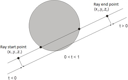
Fig. VII.13. Crossing the ray with a sphere

Let us remember that the equation of sphere with the radius r and the center in point $(l, m, n)$ has a form

$$(x-l)^2+(y-m)^2+(z-n)^2=r^2$$

Parametric equations, for $0≤t≤1$, that describe the ray starting at point $(x_1,y_1,z_1)$ and ending at point $(x_2,y_2,z_2)$ (see Fig. VII.13) may be written in the form

$$x=x_1+(x_2-x_1)t=x_1+it$$ $$y=y_1+(y_2-y_1)t=y_1+jt$$ $$z=z_1+(z_2-z_1)t=z_1+kt$$

After substituting the ray equations into sphere equation and reordering we get the quadratic equation. After finding Δ we may decide whether the ray crosses the sphere, is tangent to the sphere or does not cross a sphere at all. In the case of crossing the solution representing closer point should be chosen.

Crossing ray - triangle

Let us remember that for testing whether the point P belongs to the triangle of given vertices (A,B,C) it is possible to find barycentric coordinates of this point. If all coordinates are positive then the point belongs to the triangle.

The equation of the ray starting at point o may be written in the form (see Fig.VII.14)

$$\bi r(t)=\bi o+t\bi d$$

where d is a directional vector, usually unitary.

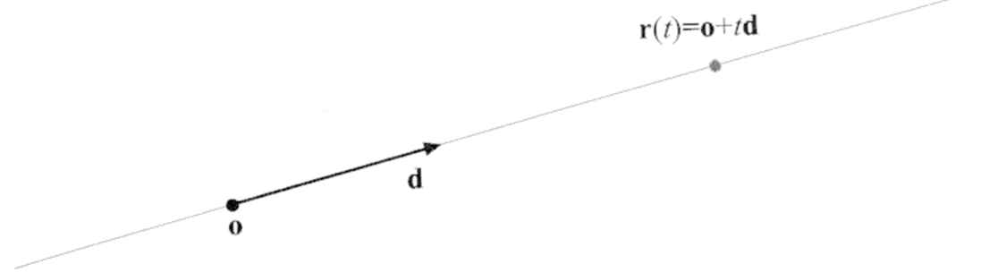
Fig. VII.14. Illustration of the method of ray description

Point P must belong to ray (for certain value of t). Hence we get a set of three equations with three unknowns α,β,t

$$\bi o+t\bi d=α\bi A+β\bi B+(1-α-β)\bi C$$