2D graphics algorithms

2D graphics

In 2D graphics during creation of the image on a plane we operate on objects such as line segments, figures or curves. These objects are described by vertices or control points and suitable attributes. The problem of objects rasterisation (presented in previous lecture) is postponed to last phase of image creation.

In relation to particular images described in vector manner different operation may be performed. Characteristic feature of these operation is that they act on vertices or on control points relevant to these objects description. The objects themselves are restored on the base of points obtained as a result of operation. Most frequently used operation acting on objects are geometric transformation: translations (shifts), revolutions, scaling and skewing.

Geometric transformations

The translation (shift) transformation of object means change of placement of all vertices by given translation vector. The example of such transformation is shown on Fig. V.1 along with the equations used in such translation. The equations enables finding the coordinates of point $(x’,y’)$ after translation about vector $T(T_x,T_y)$.

$x'=x+T_x$
$y'=y+T_y$

Fig. V.1. Translation of object about vector T

Scaling enables change of objects size with scaling coefficient S. Example of scaling is shown in Fig. V.2. At side the equations for finding new placement of point after scaling with respect to x axis and coefficient $S_x$ and with respect to y axis and coefficient $S_y$ are shown.

$x'=x·S_x$
$y'=y·S_y$

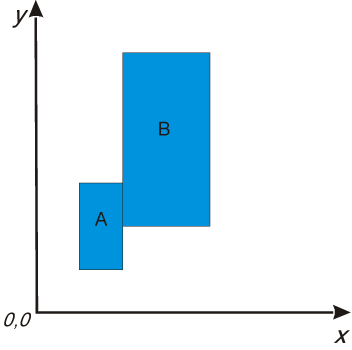
Fig. V.2. Example of object scaling with coefficients $S_x=S_y=2$. Reference point is the origin of coordinate system

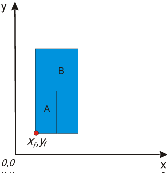
Let us notice that the reference point is s relevant in scaling operation. In Fig. V.2 reference point is the origin of coordinate system. In general reference point $x_f$, $y_f$ for scaling may be set at any place on the plane. In Fig. V.3 the example of scaling with reference point placed at lower left corner of scaled object.

$x'=x·S_x+x_f(1-S_x)$
$y'=y·S_y+y_f(1-S_y)$

Fig. V.3. Example of object scaling with coefficients $S_x=S_y=2$. Reference point is a point with coordinates $x_f=1$, $y_f=1$

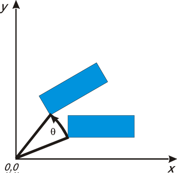
In Fig. V.4 the revolution of object about the origin of coordinate system through angle θ (revolution through positive angle is counter-clockwise) is shown. The equations for finding coordinates of points after revolution through given angle θ about the origin of coordinate system are placed right to the figure.

$x'=x\cosθ-y\sinθ$
$y'=x\sinθ+y\cosθ$

Fig. V.4. Revolution of object through given angle θ about the origin of coordinate system

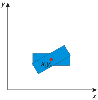
Similarly to scaling case for rotation the pivot point with coordinates $x_r$, $y_r$, about which the rotation takes place is relevant. In general it may be any point on a plane. In Fig. V.5 the example of rotation the same figure as previously is shown. The angle of revolution is the same, but pivot point is now placed in the middle of rectangle.

$x'=x_r+(x-x_r)\cosθ-(y-y_r)\sinθ$
$y'=y_r+(x-x_r)\sinθ+(y-y_r)\cosθ$

Fig. V.5. Rotation of object through the given angle θ about the point with coordinates $x_r$, $y_r$

The next useful transformation is skew along x axis with coefficient a or along y axis with coefficient b. Both types of skew are shown in Fig. V.6 along with suitable equations.

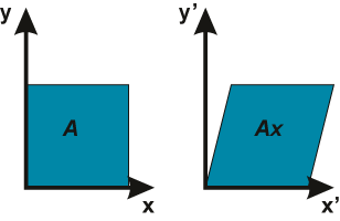
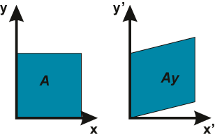
Fig. V.6. Skewing of object along x axis (Ax) and along y axis (Ay)

Homogeneous coordinates

The described above transformation in computer graphics are realized with the use so called homogeneous coordinates.

Object described in certain rectangular coordinate system, for example x,y may also be represented in coordinate system having one dimension more for example x, y, z. Then in the case of point with coordinates (a,b) we add one more coordinate that in general may have any value different form 0. If we set this new coordinate value to 1 then we accept that the point is represented in normalised homogeneous coordinates. Thus the point with coordinates (a,b) has now coordinates (a,b,1). Additionally if it would occur that in result of calculation in normalized homogeneous coordinates we would get the coordinates (a’,b’,w), we should at once make normalization step in order to get standard form with $w=1$. That means that all point coordinates should be divided by w.

Transfer to homogeneous coordinates enables uniform notation of basic geometric transformations: translation, revolution scaling and others - the most significant is inclusion of translation operation. It make easier realisation of hardware support of calculations, thus reduces the execution time.

In this approach all operation are realised in the form of multiplication of column vector representing transformed point (x,y,1) by the matrix 3 x 3 with elements suitable for performed transformation. As a result we will get coordinates of point after transformation (x’,y’,1).

The matrices for specific geometric transformations on a plane look as follows:

Translation about vector (T_x, T_y)

Scaling with scaling coefficient S_x, S_y

Revolution through angle θ about the origin of coordinate system

Skewing along x axis with coefficient a and along y with coefficient b

One of the advantages of this method of transformation representation in matrix form is that matrices for subsequent transformation can be multiplied in order to get single matrix of complex transformation. If we need to make a sequence of transformation of certain point P we may initially perform multiplication of matrices $M_i$ of next transformations (in fixed order) and get single resultant matrix M’ representing the whole sequence of transformation. It is especially computationally beneficial when the same sequence of operation is applied to great number of points, which is the usual case. The equations below explain the problem.

$P'=M_3M_2M_1P$
$M’=M_3M_2M_1$
$P’=M’P$.

If for example we would like to rotate the point not about the origin of coordinate system but about certain pivot point P(x₁,x₂), then we should make a sequence of operations. At first we should translate an object in such way that place the point P(x₁,x₂) at the origin of coordinate system, then rotate about the origin through the angle of θ, and finally move back the point from origin of coordinate system to its initial position P(x₁,x₂). That means that we should perform in a sequence: translation about vector (-x₁,-x₂), rotation through the angle of θ and translation about vector (x₁,x₂). It may be realised by three consecutive multiplications of matrix by column vector. In an equivalent method at first we prepare complex matrix that represent the concatenation of operations. Then we use this matrix to transform all objects vertices. The process of preparing complex matrix is shown below. Let us pay attention to an order of matrix notation (from right to left according to the order of performed transformations). Let us remember that in general case matrix multiplication is not alternative.

In similar manner we may find resultant matrix for another complex set of transformation. I propose to find a matrix for scaling operation with respect to the point different then the origin of coordinate system.

Clipping

Clipping operation may be necessary when the designed drawing is so big that it cannot be displayed on the screen as a whole. In such situation is reasonable to choose such fragment of the drawing that can appear on the screen and transform only these objects which will be placed in the window as a whole or at least partially. There exist a few known methods of clipping. Here we limit ourselves to discuss classic Cohen-Sutherland line clipping method and Sutherland-Hodgeman polygon clipping method.

Let us start from line segment clipping problem. The algorithm is realised in two phases. In the first phase we try to eliminate from clipping process these line segments that surely do not require any action: either they lie completely outside the window or are located fully in the window. The examples of different placement of line segments with respect to the window are shown in Fig. V.7. In second phase each of the remaining from phase 1 line segments is individually clipped.

Fig. V.7. Examples of line segments placement with respect to the clipping window

For fast testing whether the line segment may be eliminated from further clipping procedure Cohen and Sutherland proposed to divide a window plane into nine parts by extending the window edges. Each part has assigned a four bit code, what is illustrated in Fig. V.8. The principle of code assignment is as follows. All parts left to the window has „1” on the first code position. All parts right to the window has „1” on the second code position etc.

Fig. V.8. a) Division of plane into parts and method of code assignment, b) examples of analysed line segments

Decision concerning possibility of elimination of line segment is undertaken in following manner. Each endpoint has assigned a code of area where this point is placed. Then we find logical product of this codes (logical product of each bit position is performed independently). If the product is different from 0, the line segment may be discarded (for example line segment A on figure) as lying entirely outside the window. We may also eliminate from further clipping procedure these line segments that has both endpoints in the window (line segment D on figure). The remaining line segments cannot be eliminated although they for sure lie outside the window, such as line segment B on figure. Such simple procedure is not able to distinguish between line segments B and C on figure. Although the effectiveness of the procedure is not 100% it is used due to its simplicity. All line segment which have not been eliminated undergo the further clipping procedure.

Clipping procedure consists of four steps. In each step we perform clipping against the line containing one edge of a window, always in the same order. During clipping we find crosspoint of the line and line segment and reject this part of line segment which lies outside the window. Procedure is illustrated in Fig. V.9.

Fig. V.9. Clipping procedure of line segment by next lines defined by window edges

Clipping of convex polygons may be realised as follows. At first it is worth testing the placement of polygon with respect to the window. Possible cases are shown in Fig. V.10.

Fig. V.10. Possible placement of polygon with respect to the window. a) object and window are separated, b) polygon lies entirely inside the window, c) polygon crosses with window, d) window is enclosed in polygon

In the three cases the way of action is obvious. Only the c) case requires continuing the procedure. It may be realised in four steps. In each step we clip by the next window edge (precisely by the line containing the edge). At each time we reject this part of polygon that lie outside the window, as shown in Fig. V.11. In this case it was sufficient to clip by two edges of window.

Fig. V.11. Example of polygon clipping

In the simplest case in clipping procedure we may use directly the algorithm of line clipping for the edges of clipped polygon. More convenient is use of concept proposed by Sutherland and Hodgeman.

Let us assume that we will scroll the edges in the counter-clockwise direction. Let us assume also that for each line containing the edge we distinguish inner and outer side - the window lies on inner side. The idea of concept is shown on Fig. V.12. There are four situation that may appear during analysis the relation between edge of polygon with considered line. The edge of polygon may go from outer part to inner part of considered line. Then we find crossing point P and put this point P along with ending point of the edge of polygon W on auxiliary list. If the edge of polygon lies entirely on inner side of considered line we put ending point of the edge of polygon W on auxiliary list. If the edge of polygon go towards outer side of consider line the cross point with the edge of the window is put on the list. If the edge of polygon is entirely on outer side nothing is placed on list.

Fig. V.12. Four cases of placement the edge of polygon with respect to considered line. For each case the information to be put on auxiliary list are marked

In Fig. V.13 the previous example of clipping polygon against the window using described rules is shown. For simplification instead of creation of auxiliary list appropriate points are marked directly on figure, having assigned number in the order of appearance. In each step analysis starts from the edge marked by letter A. Every time after setting the auxiliary list we connect points in the order of appearance on the list: from the first to the last and to the first. The created polygon remains.

Fig. V.13. Steps of clipping algorithm

I propose to clip on Your own the polygon shown in Fig. V.14.

Fig. V.14. Example for clipping the polygon on your own

Curves in computer graphics

Curves in computer graphics are represented as:

In graphics we may found curves with different global and local features.

In the context of global features we speak about closed curves, curves with cross-points, segmented curves (Fig. V.15a), curves that interpolate points (going through given set of points) (Fig. V.15b), curves that approximate given set of points (Fig. V.15c)

Fig. V.15. Examples of curves a) segmented curve, b) interpolating curve, c) approximating curve

Among local features of curves we at first distinguish the parameters that describe continuity in tangential points of curve's segments.

In analytical approach we use the notion of parametric continuity $C^n$, for which all derivatives up to order n inclusive are the same at both sides of the segments tangential point (for example for continuity $C^1$ the equation $f_1^'(1)=f_2^'(0)$ holds, where the actual parameter value 1 corresponds to the end of first segment and the value 0 corresponds to the start point of second segment).

In the context of computer graphics the most frequently use notion is geometric continuity. Geometric continuity $G^o$ means that two curves has the common point only. Continuity $G^1$ means that the tangents at common point are collinear. Continuity $G^2$ means that two curves continuous according to $G^1$ criterium, have the same curvature in common point. (Fig. V.16).

Fig. V.16. Illustration of geometric continuities

Another local features of a curve are placement of point on curve, direction of moving along a curve, measure of travelled distance along a curve etc.

Important class of curves are polynomial curves defined by a function:

$$f(t)=a_0+a_1t+a_2t^2+...+a_nt^n=∑↙{i=0}↖n a_it^i$$

Polynomial function may be also described in the form:

$$f(t)=∑↙{i=0}↖n c_ib_i(t)$$

where $b_i(t)$ are the polynomials specified as base polynomials in the form depending on the type of curve. When we choose appropriate set of base polynomial, coefficients $c_i$ enables the control of the shape of curve. The example are Bezier curves.

Bezier curves

Bezier curves are polynomial curves. Their shape may be described by so called control points.

The equations describing Bezier curves are written in parametric form.

where $P_k$ are control points and $B_{k,n}(u)$ are base functions (so called Bernstein polynomials) associated with certain control points.

In general case the number of control points is not limited - but the greater the number of control points the greater is the order of polynomial describing the curve. In practice the most frequently used are third order curves defined by four control points. Next we will limit ourselves to discuss exactly such curves.

In Fig. V.17 some examples of Bezier curves defined by four control points are shown.

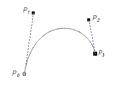
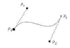
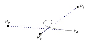
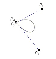
Fig. V.17. Examples of Bezier curves

Looking at shown examples we may notice a few common Bezier curves features. The order of control points is important. Curve always contains the first and the last points. The line segment connecting two first control points is always tangent to curve at the beginning point. Similarly the line segment connecting to last two control points is tangent to the curve at ending point. Moreover it is worth pointing that the curve always lies inside the polygon described on a whole set of control points. It is possible to create closed curves. Moving any control point influences the whole shape of a curve - it makes curve edition easier.

Equation of the third order curve has the form.

$$P(u)=(1-u)^3P_0+3u(1-u)^2P_1+3u^2(1-u)P_2+u^3P_3$$

Current parameter u appearing in the equation changes along the curve from the value 0 at the beginning to the value 1 at the end of a curve. Points $P_k$, k = 0,1,2,3 are curve control points. Diagrams of base functions are shown in the Fig. V.18. It is worth noting that each base function influence more or less the shape of the curve in the full range of change of parameter u.

Fig V.18. Base functions for Bezier curves defined by four control points. The value of parameter u is on horizontal axis.

It is possible to create more complex Bezier curves by joining the segments. The example is shown in Fig. V.19. Let us pay attention to curve continuity at segment joining points. The necessary condition to get continuity is that two last control points of one segment (P_a2, P_a3 in figure) lie on the same line as two first control points of the next segment (P_b0, P_b1 in figure), while the last point of first segment P_a3 overlap the first point of the next segment P_b0.

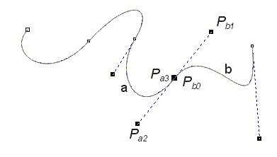
Fig. V.19. Example of Bezier curves consisting of four segments

Tools in 2D computer graphics application programs

In this lecture we have learned a few basic algorithms used in 2D graphics. These algorithms are used in different graphics application programs. Each of these programs make available tools that make easier the creation of particular objects and whole images. Sets of available tools are different in different programs. In the case of most of programs discussed all tools and the methods of application are described in extensive reference books and as a rule requires direct use of the program.

During laboratory classes we will meet professional graphics application program Corel Draw. Description of the tools may be found in reference book for present version of the program. Of course it is always possible to use „Help” available in program.